
Semimetal de Weyl deformado#
En esta sección se presenta el resultado de nuestra investigación, el cual es la introducción perturbación de nuestro semimetal de Weyl de manera mécanica.
Show code cell source
from pylab import *
mpl.rcParams.update({'font.size':18})

from plotly.subplots import make_subplots

import plotly.graph_objects  as go
import plotly.figure_factory as ff

from pythtb import * # import TB model class

from ipywidgets import interact, interactive, fixed, interact_manual
import ipywidgets as widgets
Show code cell source
import glob
from matplotlib.ticker import (MultipleLocator,
                               FormatStrFormatter,
                               AutoMinorLocator)
mpl.rcParams.update({'font.size': 22, 'text.usetex': True})
mpl.rcParams.update({'axes.linewidth':1.5})
mpl.rcParams.update({'axes.labelsize':'large'})
mpl.rcParams.update({'xtick.major.size':12})
mpl.rcParams.update({'xtick.minor.size':6})
mpl.rcParams.update({'ytick.major.size':12})
mpl.rcParams.update({'ytick.minor.size':6})
mpl.rcParams.update({'xtick.major.width':1.5})
mpl.rcParams.update({'xtick.minor.width':1.0})
mpl.rcParams.update({'ytick.major.width':1.5})
mpl.rcParams.update({'ytick.minor.width':1.0})
Hamiltoniano del sistema#
Show code cell source
from palettable.cubehelix import Cubehelix
palette = Cubehelix.make(start=-0.5, rotation=0.3,reverse=True,n=10)
---------------------------------------------------------------------------
ModuleNotFoundError                       Traceback (most recent call last)
Cell In[3], line 1
----> 1 from palettable.cubehelix import Cubehelix
      2 palette = Cubehelix.make(start=-0.5, rotation=0.3,reverse=True,n=10)

ModuleNotFoundError: No module named 'palettable'
Show code cell source
#Parámetros
a  = 1.0
k_0= pi/2

tx = 1
t  = 1
m  = 2*t
γ  = 0

A_x= 0.0
A_y= +0.0
A_z= 0.0

##################----------------Inicia TB----------------##################
lat= [[a,0,0],[0,a,0],[0,0,a]]
orb= [[0,0,0],[1/2,1/2,1/2]] #H, solo los sitios A[000] B1/2[111]

WSH = tb_model(3,3,lat,orb)

#DIAGONAL
#γ*(cos(k_x)-cos(k_0))-2*t*sin(k_z)
# γ[coskx]
WSH.set_hop( γ/2, 0, 0,[1,0,0])#de que sitio a que sitio va el hoping, [la exp que lleva ese parametro], Conjugado ya no es
# -2tsinkz                                #necesario, está implícito porque es Hermitiano.
WSH.set_hop(-t/1J, 0, 0,[0,0,1])

#Hermitiano [1,1]
WSH.set_hop(γ/2, 1, 1,[1,0,0])
WSH.set_hop(t/1J, 1, 1,[0,0,1])

WSH.set_onsite([-γ*cos(k_0),-γ*cos(k_0)]) # No hay hooping, es energia

#FUERA DE LA DIAGONAL

# -[m*(2-cos(k_y)-cos(k_z))+2*tx*(cos(k_x)-cos(k_0))]+2J*t*sin(k_y)
#  2txcosk_0
WSH.set_hop(-2*m+2*(tx)*cos(k_0), 0, 1,[0,0,0])
#mcosky+ 2itsin(ky)
WSH.set_hop(m/2+t, 0, 1,[0, 1,0])
WSH.set_hop(m/2-t, 0, 1,[0,-1,0])
# WSH.set_hop(m/2-t, 1, 0,[0,+1,0])
# mcoskz
WSH.set_hop(m/2, 0, 1,[0,0,1])
WSH.set_hop(m/2, 0, 1,[0,0,-1])
# tx(coskx)
WSH.set_hop(-tx+A_x, 0, 1,[1,0,0])
WSH.set_hop(-tx+A_x, 0, 1,[-1,0,0])
Introducción del Strain en el Hamiltoniano#
Los hopping los modificaremos de la siguiente forma.
donde \(a_{\text{nn}}\) es la distancia de equilibrio.
Show code cell source
"""La siguiente función permite obtener la DOS usando Funciones de Green"""
Et=linspace(-10,13,1001)
def G(Edos):
    GreenP = []
    f      = 0.01 #al aumentarlo, mejora la fidelidad al hsitograma

    for i in Et:
        g  = sum(1/(i+f*1J-Edos))
        GreenP.append(g)
    GreenM = []

    for i in Et:
        g  = sum(1/(i-f*1J-Edos))
        GreenM.append(g)

    GIP  = -imag(GreenP)
    GRP  = real(GreenP)

    return GIP, GRP
Show code cell source
"""Construccion de la malla para un sistema de PR*PR puntos k"""
PR    = 101
kx,ky = linspace(0,1,PR),linspace(0,1,PR)
KX,KY = meshgrid(kx,ky)
KX,KY = KX.flatten(),KY.flatten()
Kf         = column_stack((KX,KY))
# solve the model on this mesh
# Ekf=N_WSM.solve_all(Kf)
# # flatten completely the matrix
# Ekf=Ekf.flatten()
Show code cell source
""""La siguiente función permite aplicar el strain de una funcion u(Y) al sistema que es una malla de PR*PR puntos k
Los argumentos son: epsilon, β, la funcion de deformación y el plano en Z que se estudia"""

def StrainKF(eps,beta,funstrain,z):

    uY   = (eps/L)*funstrain
    Ynew = Y + uY

    pares=arange(0,2*L,2)
    nones=arange(3,2*L,2)

    for l in range(L-1):
        hop1 = (m/2+t)*exp(beta*(1 - (Ynew[nones[l]]-Ynew[pares[l]])/((Y[nones[l]]-Y[pares[l]]))  ))
        NY_WSM.set_hop(hop1,pares[l],nones[l],[0,0,0],mode='reset')
    for p in pares[1:]:
        hop2 = (m/2-t)*exp(beta*(1 - (Ynew[p]-Ynew[p-1])/(Y[p]-Y[p-1])  ))
        NY_WSM.set_hop(hop2,p,p-1,[0,0,0],mode='reset')

#     k = [[0.0,z],[0.5,z],[1,z]] # Punto por los cuales que quiero que pase. Son los punto de al simetria
#                                  #unidades en unidades de V de red 1=2pi/a
#     k_label=[r"$-X$",r"$\Gamma$",r"$X$"]
#     (k_vec,k_dist,k_node)=NY_WSM.k_path(k,501,report=False)
    Ek,ψ =NY_WSM.solve_all(Kf,eig_vectors=True)
#     (k_vec,k_dist,k_node)=NZ_WSM.k_path(k,501,report=False)
#     Ek1,ψ1 =NZ_WSM.solve_all(k_vec,eig_vectors=True)
#     fig,ax=plt.subplots(ncols=2,nrows=1,figsize=(16,8),
#                        gridspec_kw = {'wspace':0.2, 'hspace':0.4, 'width_ratios': [1,1]})
#     for l in range(len(Ek)):
#          a=ax[0].plot(k_dist,Ek[l,:], c='black', alpha=0.6)
#          b=ax[1].plot(k_dist,Ek1[l,:], c='purple', alpha=0.6)
    return Ek, ψ, max(uY)
Show code cell source
""""La siguiente función permite aplicar el strain de una funcion u(Y) al sistema que es una maya de PR*PR puntos k
Los argumentos son: epsilon, β, la funcion de deformación y el plano en Z que se estudia.

A diferencia de la anterior en este el numero de puntos k es de 501"""

def Strain(eps,beta,funstrain,z):

    uY   = (eps/L)*funstrain
    Ynew = Y + uY

    pares=arange(0,2*L,2)
    nones=arange(3,2*L,2)

    for l in range(L-1):
        hop1 = (m/2+t)*exp(beta*(1 - (Ynew[nones[l]]-Ynew[pares[l]])/((Y[nones[l]]-Y[pares[l]]))  ))
        NY_WSM.set_hop(hop1,pares[l],nones[l],[0,0,0],mode='reset')
    for p in pares[1:]:
        hop2 = (m/2-t)*exp(beta*(1 - (Ynew[p]-Ynew[p-1])/(Y[p]-Y[p-1])  ))
        NY_WSM.set_hop(hop2,p,p-1,[0,0,0],mode='reset')

    k = [[0.0,z],[0.5,z],[1,z]] # Punto por los cuales que quiero que pase. Son los punto de al simetria
                                 #unidades en unidades de V de red 1=2pi/a
    k_label=[r"$-X$",r"$\Gamma$",r"$X$"]
    (k_vec,k_dist,k_node)=NY_WSM.k_path(k,501,report=False)
    Ek,ψ =NY_WSM.solve_all(k_vec,eig_vectors=True)
#     (k_vec,k_dist,k_node)=NZ_WSM.k_path(k,2001,report=False)
#     Ek1,ψ1 =NZ_WSM.solve_all(k_vec,eig_vectors=True)
#     fig,ax=plt.subplots(ncols=2,nrows=1,figsize=(16,8),
#                        gridspec_kw = {'wspace':0.2, 'hspace':0.4, 'width_ratios': [1,1]})
#     for l in range(len(Ek)):
#          a=ax[0].plot(k_dist,Ek[l,:], c='black', alpha=0.6)
#          b=ax[1].plot(k_dist,Ek1[l,:], c='purple', alpha=0.6)
    return Ek, ψ, max(uY)
Show code cell source
"""Esta función permite obtner el IPR dando los eigenestados del sistema"""


def IPR(ψk):
    nBands,nkpts,nsites= shape(ψk)
    I     = []
    ik =nkpts//2
    prob=0
    for i in range((nsites)):
        prob +=( conj(ψk[i][ik])*ψk[i][ik])**4
        suma2=  vdot(ψk[i][ik],ψk[i][ik])**2

    I=array((prob/suma2).real)
    return I
Show code cell source
"""Construcción del sistema finito"""
L=101
NY_WSM=WSH.cut_piece(L,1,glue_edgs=False) #numero de reps, en la direccion 0x,1y,2z, mi sistema se redujo dimensionalmente                                        #modo rebanada de jamón
NYN_WSM=WSH.cut_piece(L,1,glue_edgs=False)
Show code cell source
"""Obtención de las coordenadas de los motivos de la red (cubica)"""

X,Y,Z = dot( NY_WSM.get_orb(), NY_WSM.get_lat() ).T

eps=15
n=12
beta=2
funstrain=cos(n*pi*Y/L)
uY   = (eps/L)*funstrain
Ynew = Y + uY
Show code cell source
Ek6s,ψ6s,max_u6s= Strain(eps,beta, funstrain,0.0)
z=0
k = [[0.0,z],[0.5,z],[1,z]] # Punto por los cuales que quiero que pase. Son los punto de al simetria
                                 #unidades en unidades de V de red 1=2pi/a
k_label=[r"$-X$",r"$\Gamma$",r"$X$"]

(k_vec,k_dist,k_node)=NYN_WSM.k_path(k,501,report=False)
Ek0,ψ0 =NYN_WSM.solve_all(k_vec,eig_vectors=True)
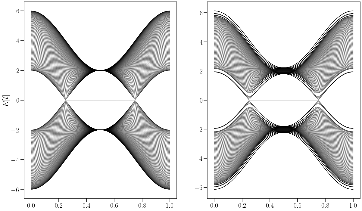
Comparación de un sistema tipico de WSM tipo I no perturbado con un sistema perturbado.#
fig,ax  = plt.subplots(ncols=2,nrows=1,figsize=(20,12),
                       gridspec_kw = {'wspace':0.2, 'hspace':0.4, 'width_ratios': [1,1]})
k_dist=linspace(0,1,501)
for n in range(0, len(Ek0)):

    ax[0].plot(k_dist,Ek0[n,:], c='black', alpha=0.6,linewidth=1.1) #la long de Ek fin tiene todo
    ax[1].plot(k_dist,Ek6s[n,:], c='black', alpha=0.6,linewidth=1.1)


ax[0].set_ylabel(r"$E[t]$",fontsize=26)
ax[0].set_ylabel(r"$E[t]$",fontsize=26)

savefig("LatChemStrai_cos(na)_WSM_TII.pdf", bbox_inches="tight")
Show code cell source
prob=IPR(ψ6s)
shape(prob)

prob
array([0.125, 1.   , 0.125, 0.125, 0.125, 0.125, 0.125, 0.125, 0.125,
       0.125, 0.125, 0.125, 0.125, 0.125, 0.125, 0.125, 0.125, 0.125,
       0.125, 0.125, 0.125, 0.125, 0.125, 0.125, 0.125, 0.125, 0.125,
       0.125, 0.125, 0.125, 0.125, 0.125, 0.125, 0.125, 0.125, 0.125,
       0.125, 0.125, 0.125, 0.125, 0.125, 0.125, 0.125, 0.125, 0.125,
       0.125, 0.125, 0.125, 0.125, 0.125, 0.125, 0.125, 0.125, 0.125,
       0.125, 0.125, 0.125, 0.125, 0.125, 0.125, 0.125, 0.125, 0.125,
       0.125, 0.125, 0.125, 0.125, 0.125, 0.125, 0.125, 0.125, 0.125,
       0.125, 0.125, 0.125, 0.125, 0.125, 0.125, 0.125, 0.125, 0.125,
       0.125, 0.125, 0.125, 0.125, 0.125, 0.125, 0.125, 0.125, 0.125,
       0.125, 0.125, 0.125, 0.125, 0.125, 0.125, 0.125, 0.125, 0.125,
       0.125, 0.125, 0.125, 0.125, 0.125, 0.125, 0.125, 0.125, 0.125,
       0.125, 0.125, 0.125, 0.125, 0.125, 0.125, 0.125, 0.125, 0.125,
       0.125, 0.125, 0.125, 0.125, 0.125, 0.125, 0.125, 0.125, 0.125,
       0.125, 0.125, 0.125, 0.125, 0.125, 0.125, 0.125, 0.125, 0.125,
       0.125, 0.125, 0.125, 0.125, 0.125, 0.125, 0.125, 0.125, 0.125,
       0.125, 0.125, 0.125, 0.125, 0.125, 0.125, 0.125, 0.125, 0.125,
       0.125, 0.125, 0.125, 0.125, 0.125, 0.125, 0.125, 0.125, 0.125,
       0.125, 0.125, 0.125, 0.125, 0.125, 0.125, 0.125, 0.125, 0.125,
       0.125, 0.125, 0.125, 0.125, 0.125, 0.125, 0.125, 0.125, 0.125,
       0.125, 0.125, 0.125, 0.125, 0.125, 0.125, 0.125, 0.125, 0.125,
       0.125, 0.125, 0.125, 0.125, 0.125, 0.125, 0.125, 0.125, 0.125,
       0.125, 0.125, 1.   , 0.125])
Ubicación de los arcos de Fermi: estados de superficie o borde#
Show code cell source
fig,ax = plt.subplots(figsize=(7,6))
colores = ["r", "b", "g"]
# ax.scatter(X,Y,c="blue")000
triang = ax.scatter(X,Ynew,c=log(prob),cmap=cm.plasma_r,s=prob*50, vmin=-4, vmax=log(1), alpha=0.8)
for i in range(50):
    ax.scatter(X+i,Ynew,c=log(prob),cmap=cm.plasma_r,s=prob*50, vmin=-4, vmax=log(1), alpha=0.8)

plt.colorbar(triang,ax=ax,label="$Log_{10}\;|\psi|^4$")
ax.set_ylabel("$Y$")
ax.set_xlabel("$X$")
savefig("UbiFermiArcs.pdf", bbox_inches= "tight")
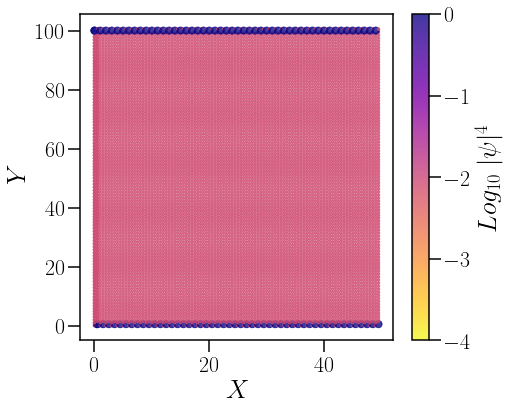
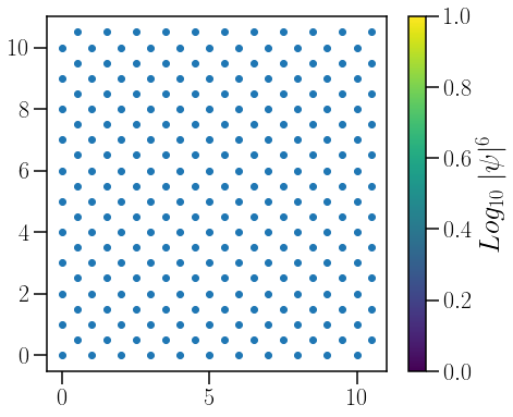
En la figura anterior se puede denotar que los estados electrónicos más localizados se encuentran en los bordes del material. De estudios anteriores sabemos que los arcos de Fermi son los estados con mayor localuzación, por lo que podemos concluir que dichos estados de superficie corresponden a los arcos de Fermi.
Evolución del sistema perturbado al aumentar el parámetro de deformación \(n\)#
%%time
e=15
Ek1,ψ1,max_u1= Strain(0,2, cos(2*pi*Y/L),0.0)
Ek2,ψ2,max_u2= Strain(e,2, cos(2*pi*Y/L),0.0)
Ek3,ψ3,max_u3= Strain(e,2, cos(4*pi*Y/L),0.0)
Ek4,ψ4,max_u4= Strain(e,2, cos(6*pi*Y/L),0.0)
Ek5,ψ5,max_u5= Strain(e,2, cos(10*pi*Y/L),0.0)
Ek6,ψ6,max_u6= Strain(e,2, cos(12*pi*Y/L),0.0)
CPU times: user 1min 24s, sys: 584 ms, total: 1min 24s
Wall time: 1min 24s
fig,ax  = plt.subplots(ncols=3,nrows=2,figsize=(20,12),
                       gridspec_kw = {'wspace':0.4, 'hspace':0.4, 'width_ratios': [1,1,1]})
k_dist=linspace(0,1,501)
for n in range(0, len(Ek1)):

    ax[0,0].plot(k_dist,Ek1[n,:], c='black', alpha=0.6,linewidth=1.1) #la long de Ek fin tiene todo
    ax[0,1].plot(k_dist,Ek2[n,:], c='black', alpha=0.6,linewidth=1.1)
    ax[0,2].plot(k_dist,Ek3[n,:], c='black', alpha=0.6,linewidth=1.1)#la long de Ek fin tiene todo
    ax[1,0].plot(k_dist,Ek4[n,:], c='black', alpha=0.6,linewidth=1.1)
    ax[1,1].plot(k_dist,Ek5[n,:] ,c='black', alpha=0.6,linewidth=1.1 )
    ax[1,2].plot(k_dist,Ek6[n,:], c='black', alpha=0.6,linewidth=1.1)

for i in range(0,2):
    for j in range(0,3):
        ax[i,j].spines['right'].set_visible(False)
        ax[i,j].spines['top'].set_visible(False)
#         ax[i,j].set_ylim(-1,1)

ax[0,0].set_ylabel(r"$E[t]$",fontsize=26)
ax[1,0].set_ylabel(r"$E[t]$",fontsize=26)

ax[0,0].set_xlabel(r"Finito en Y, $S=cos(2g)|u_m={0}$".format(0.15),fontsize=26)
ax[0,1].set_xlabel(r"Finito en Y, $S=cos(4g)|u_m={0}$".format(0.15),fontsize=26)
ax[0,2].set_xlabel(r"Finito en Y, $S=cos(6g)|u_m={0}$".format(0.15),fontsize=26)
ax[1,0].set_xlabel(r"Finito en Y, $S=cos(8g)|u_m={0}$".format(0.15),fontsize=26)
ax[1,1].set_xlabel(r"Finito en Y, $S=cos(10g)|u_m={0}$".format(0.15),fontsize=26)
ax[1,2].set_xlabel(r"Finito en Y, $S=cos(12g)|u_m={0}$".format(0.15),fontsize=26)
savefig("LatChemStrai_cos(na)_WSM_TII.pdf", bbox_inches="tight")
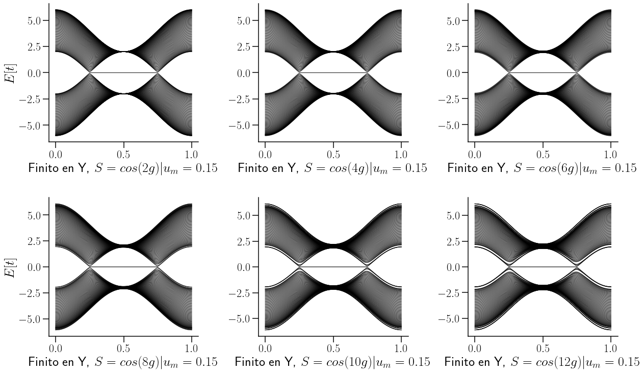
Se puede obseervar que conforme aumenta el parámetro de deformación se va abriendo un gap alrededor de los nodos de Weyl, y los estados alrededor de \(k=\)0.5 se van concentrando.
Show code cell source
e=15
Ek1s,ψ1s,max_u1s= Strain(e,2, sin(2*pi*Y/L),0.0) #esp, beta, función de strain
Ek2s,ψ2s,max_u2s= Strain(e,2, sin(4*pi*Y/L),0.0)
Ek3s,ψ3s,max_u3s= Strain(e,2, sin(6*pi*Y/L),0.0)
Ek4s,ψ4s,max_u4s= Strain(e,2, sin(8*pi*Y/L),0.0)
Ek5s,ψ5s,max_u5s= Strain(e,2, sin(10*pi*Y/L),0.0)
Ek6s,ψ6s,max_u6s= Strain(e,2, sin(12*pi*Y/L),0.0)
Show code cell source
Ek6s,ψ6s,max_u6s= StrainKF(e,2, sin(12*pi*Y/L),0.0)
Ek0,ψ0,max_u0= StrainKF(0,2,sin(12*pi*Y/L),0.0)
Show code cell source
GStrain,GN= G(Ek6s),G(Ek0)
¿Cómo se ve afectada la densidad de estados?#
Show code cell source
fig,ax  = plt.subplots(ncols=2,nrows=1,figsize=(16,6),
                       gridspec_kw = {'wspace':0.2, 'hspace':0., 'width_ratios': [1,1]})
Na=1/(101*101*100*6.27)
ax[0].plot(Et,GStrain[0]*Na,color="red", alpha=0.9,label="Strained TI WSM.")
ax[0].plot(Et,GN[0]*Na, alpha=0.5,label="Non-perturbed TI WSM")
ax[0].set_xlim(-10,10)
ax[0].legend(loc=0,fontsize=12)

ax[1].plot(Et,GStrain[0]*Na,color="red", alpha=0.9)
ax[1].plot(Et,GN[0]*Na, alpha=0.5)
a=4
ax[1].set_xlim(-a,a)
ax[1].set_ylim(0.075,0.15)
ax[1].set_xlabel("Band energy")
ax[0].set_xlabel("Band energy")
ax[0].set_ylabel("Number of states")
ax[1].spines['right'].set_visible(False)
ax[1].spines['top'].set_visible(False)
ax[0].spines['right'].set_visible(False)
ax[0].spines['top'].set_visible(False)
savefig("strainDOS-WMSTI.pdf",bbox_inches="tight")
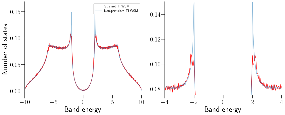
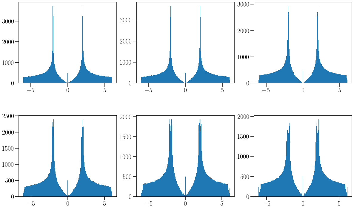
La DOS pierde la singularidad de Van Hove, como consecuencia de la perturbación mecánica.
Show code cell source
a=trapz(GStrain[0]/(101*101*100*6.27), Et)
a
1.0109347802613633
e=15
Ek1s,ψ1s,max_u1s= Strain(e,2, sin(2*pi*Y/L),0.0) #esp, beta, función de strain
Ek2s,ψ2s,max_u2s= Strain(e,2, sin(4*pi*Y/L),0.0)
Ek3s,ψ3s,max_u3s= Strain(e,2, sin(6*pi*Y/L),0.0)
Ek4s,ψ4s,max_u4s= Strain(e,2, sin(8*pi*Y/L),0.0)
Ek5s,ψ5s,max_u5s= Strain(e,2, sin(10*pi*Y/L),0.0)
Ek6s,ψ6s,max_u6s= Strain(e,2, sin(12*pi*Y/L),0.0)
Show code cell source
fig,ax  = plt.subplots(ncols=3,nrows=2,figsize=(20,12),
                       gridspec_kw = {'wspace':0.2, 'hspace':0.4, 'width_ratios': [1,1,1]})
for n in range(0, len(Ek1s)):

    ax[0,0].plot(k_dist,Ek1s[n,:], c='black', alpha=0.6,linewidth=1.1) #la long de Ek fin tiene todo
    ax[0,1].plot(k_dist,Ek2s[n,:], c='black', alpha=0.6,linewidth=1.1)
    ax[0,2].plot(k_dist,Ek3s[n,:], c='black', alpha=0.6,linewidth=1.1)#la long de Ek fin tiene todo
    ax[1,0].plot(k_dist,Ek4s[n,:], c='black', alpha=0.6,linewidth=1.1)
    ax[1,1].plot(k_dist,Ek5s[n,:] ,c='black', alpha=0.6,linewidth=1.1 )
    ax[1,2].plot(k_dist,Ek6s[n,:], c='black', alpha=0.6,linewidth=1.1)

for i in range(0,2):
    for j in range(0,3):
        ax[i,j].spines['right'].set_visible(False)
        ax[i,j].spines['top'].set_visible(False)

ax[0,0].set_ylabel(r"$E[t]$",fontsize=26)
ax[1,0].set_ylabel(r"$E[t]$",fontsize=26)

ax[0,0].set_xlabel(r"Finito en Y, $S=sin(2g)|u_m={0}$".format(0.15),fontsize=26)
ax[0,1].set_xlabel(r"Finito en Y, $S=sin(4g)|u_m={0}$".format(0.15),fontsize=26)
ax[0,2].set_xlabel(r"Finito en Y, $S=sin(6g)|u_m={0}$".format(0.15),fontsize=26)
ax[1,0].set_xlabel(r"Finito en Y, $S=sin(8g)|u_m={0}$".format(0.15),fontsize=26)
ax[1,1].set_xlabel(r"Finito en Y, $S=sin(10g)|u_m={0}$".format(0.15),fontsize=26)
ax[1,2].set_xlabel(r"Finito en Y, $S=sin(12g)|u_m={0}$".format(0.15),fontsize=26)
savefig("Strain_sin_WSM_TII.pdf", bbox_inches="tight")
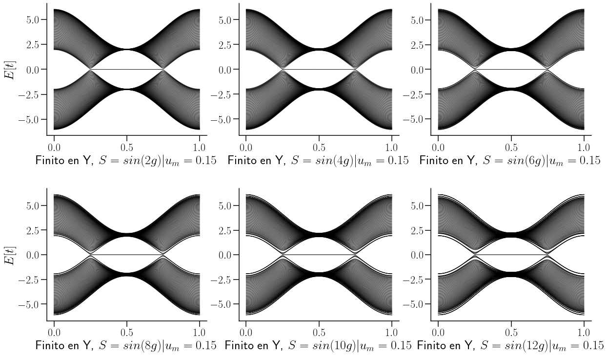
No importa si la funciín de deformación es un \( \sin\) o \(\cos\), el efecto sobre la estructura de bandas es el mismo, al igual que sobre la densidad de estados. Véase siguiente figura:
fig,ax  = plt.subplots(ncols=3,nrows=2,figsize=(20,12),
                       gridspec_kw = {'wspace':0.2, 'hspace':0.4, 'width_ratios': [1,1,1]})
a=201

ax[0,0].hist(Ek1.flatten(),a);
ax[0,1].hist(Ek2.flatten(),a);
ax[0,2].hist(Ek3.flatten(),a);
ax[1,0].hist(Ek4.flatten(),a);
ax[1,1].hist(Ek5.flatten(),a);
ax[1,2].hist(Ek6.flatten(),a);
Obtención del IPR#
Ik2=IPR(ψ2)

Ik4=IPR(ψ4)

Ik6=IPR(ψ6)
# Ik1s=IPR(ψ1s)
# Ik2s=IPR(ψ2s)
# Ik3s=IPR(ψ3s)
# Ik4s=IPR(ψ4s)
# Ik5s=IPR(ψ5s)
shape(Ik2)
# Ik6s=IPR(ψ6s)
(202,)
fig,ax  = plt.subplots(ncols=3,nrows=1,figsize=(28,7),
                       gridspec_kw = {'wspace':0.2, 'hspace':0.4, 'width_ratios': [1,1,1]})
k_dist=linspace(0,1,2001)
for n in range(0, len(Ek2)):

    Ekval=Ek2[n,:]
    amp  =Ik2[n]
    ax[0].scatter(k_dist,Ekval,c =log10(amp), vmin=-3,vmax=0, cmap = 'cubehelix_r',s = 0.5, alpha=0.5,rasterized=True)

    Ekval=Ek4[n,:]
    amp  =Ik4[n,:]
    ax[2].scatter(k_dist,Ekval,c =log10(amp), vmin=-3,vmax=0, cmap = 'cubehelix_r',s = 0.5, alpha=0.5,rasterized=True)

    Ekval=Ek6[n,:]
    amp  =Ik6[n,:]
    ax[1].scatter(k_dist,Ekval,c =log10(amp), vmin=-3,vmax=0, cmap = 'cubehelix_r',s = 0.5, alpha=0.5,rasterized=True)


for i in range(0,3):
    ax[i].spines['right'].set_visible(False)
    ax[i].spines['top'].set_visible(False)
    ax[i].set_ylim(-1.8,1.8)
#     ax[i].set_xlim(0,1)


ax[0].set_ylabel(r"$E[t]$",fontsize=26)
# ax[1,0].set_ylabel(r"$E[t]$",fontsize=26)

# ax[0,0].set_xlabel(r"Finito Y, $S=cos(2g)|u_m={0}$".format(max_u1s),fontsize=26)
# ax[0,1].set_xlabel(r"Finito Y, $S=cos(4g)|u_m={0}$".format(max_u2s),fontsize=26)
# ax[0,2].set_xlabel(r"Finito Y, $S=cos(6g)|u_m={0}$".format(max_u3s),fontsize=26)
# ax[1,0].set_xlabel(r"Finito Y, $S=cos(8g)|u_m={0}$".format(round(max_u4s,2)),fontsize=26)
# ax[1,1].set_xlabel(r"Finito Y, $S=cos(10g)|u_m={0}$".format(max_u5s),fontsize=26)
# ax[1,2].set_xlabel(r"Finito Y, $S=cos(12g)|u_m={0}$".format(max_u6s),fontsize=26)

savefig("LatchemStrain_IPR_cos_WSM_TII.pdf", bbox_inches="tight")
---------------------------------------------------------------------------
IndexError                                Traceback (most recent call last)
<ipython-input-51-26eb5bafb7f7> in <module>
      5
      6     Ekval=Ek2[n,:]
----> 7     amp  =Ik2[n,:]
      8     ax[0].scatter(k_dist,Ekval,c =log10(amp), vmin=-3,vmax=0, cmap = 'cubehelix_r',s = 0.5, alpha=0.5,rasterized=True)
      9

IndexError: too many indices for array
%matplotlib inline
k_dist=linspace(0,1,10201)
len(k_dist)
10201
shape(Ek2)
(200, 10201)
fig,ax  = plt.subplots(ncols=3,nrows=2,figsize=(20,12),
                       gridspec_kw = {'wspace':0.2, 'hspace':0.4, 'width_ratios': [1,1,1]})
for n in range(0, len(Ek1s)):
    Ekval=Ek1s[n,:]
    amp  =Ik1s[n,:]
    ax[0,0].scatter(k_dist,Ekval,c =log10(amp), vmin=-3,vmax=0, cmap = 'cubehelix_r',s = 0.5, alpha=0.5,rasterized=True)
    Ekval=Ek2s[n,:]
    amp  =Ik2s[n,:]
    ax[0,1].scatter(k_dist,Ekval,c =log10(amp), vmin=-3,vmax=0, cmap = 'cubehelix_r',s = 0.5, alpha=0.5,rasterized=True)
    Ekval=Ek3s[n,:]
    amp  =Ik3s[n,:]
    cmap = ax[0,2].scatter(k_dist,Ekval,c =log10(amp), vmin=-3,vmax=0, cmap = 'cubehelix_r',s = 0.5, alpha=0.5,rasterized=True)
    Ekval=Ek4s[n,:]
    amp  =Ik4s[n,:]
    ax[1,0].scatter(k_dist,Ekval,c =log10(amp), vmin=-3,vmax=0, cmap = 'cubehelix_r',s = 0.5, alpha=0.5,rasterized=True)
    Ekval=Ek5s[n,:]
    amp  =Ik5s[n,:]
    ax[1,1].scatter(k_dist,Ekval,c =log10(amp), vmin=-3,vmax=0, cmap = 'cubehelix_r',s = 0.5, alpha=0.5,rasterized=True)
    Ekval=Ek6s[n,:]
    amp  =Ik6s[n,:]
    ax[1,2].scatter(k_dist,Ekval,c =log10(amp), vmin=-3,vmax=0, cmap = 'cubehelix_r',s = 0.5, alpha=0.5,rasterized=True)


for i in range(0,2):
    for j in range(0,3):
        ax[i,j].spines['right'].set_visible(False)
        ax[i,j].spines['top'].set_visible(False)

ax[0,0].set_ylabel(r"$E[t]$",fontsize=26)
ax[1,0].set_ylabel(r"$E[t]$",fontsize=26)

ax[0,0].set_xlabel(r"Finito Y, $S=sin(2g)|u_m={0}$".format(max_u1s),fontsize=26)
ax[0,1].set_xlabel(r"Finito Y, $S=sin(4g)|u_m={0}$".format(max_u2s),fontsize=26)
ax[0,2].set_xlabel(r"Finito Y, $S=sin(6g)|u_m={0}$".format(max_u3s),fontsize=26)
ax[1,0].set_xlabel(r"Finito Y, $S=sin(8g)|u_m={0}$".format(round(max_u4s,2)),fontsize=26)
ax[1,1].set_xlabel(r"Finito Y, $S=sin(10g)|u_m={0}$".format(max_u5s),fontsize=26)
ax[1,2].set_xlabel(r"Finito Y, $S=sin(12g)|u_m={0}$".format(max_u6s),fontsize=26)
fig.colorbar(cmap)
savefig("Strain_IPR_sin_WSM_TI.pdf", bbox_inches="tight")
Nuevo corte en Z: Visualización de los arcos de fermi#
"""Construcción del sistema finito"""
L=21
NY_WSM=WSH.cut_piece(L,1,glue_edgs=False) #numero de reps, en la direccion 0x,1y,2z, mi sistema se redujo dimensionalmente                                        #modo rebanada de jamón

"""Obtención de las coordenadas de los motivos de la red (cubica)"""

X,Y,Z = dot( NY_WSM.get_orb(), NY_WSM.get_lat() ).T
NYZ_WSM  = NY_WSM.cut_piece(L,2,glue_edgs=False)
# NYZX_WSM = NYZ_WSM.cut_piece(L,0,glue_edgs=False)
eps=15
n=12
beta=2
funstrain=cos(n*pi*Y/L)
uY   = (eps/L)*funstrain
Ynew = Y + uY

pares=arange(0,2*L,2)
nones=arange(3,2*L,2)

for l in range(L-1):
    hop1 = (m/2+t)*exp(beta*(1 - (Ynew[nones[l]]-Ynew[pares[l]])/((Y[nones[l]]-Y[pares[l]]))  ))
    NY_WSM.set_hop(hop1,pares[l],nones[l],[0,0,0],mode='reset')
for p in pares[1:]:
    hop2 = (m/2-t)*exp(beta*(1 - (Ynew[p]-Ynew[p-1])/(Y[p]-Y[p-1])  ))
    NY_WSM.set_hop(hop2,p,p-1,[0,0,0],mode='reset')

# Ek,ψ =NY_WSM.solve_all(Kf,eig_vectors=True)
k = [[0.0],[0.5],[1]] # Punto por los cuales que quiero que pase. Son los punto de al simetria
                                 #unidades en unidades de V de red 1=2pi/a
k_label=[r"$-X$",r"$\Gamma$",r"$X$"]
(k_vec,k_dist,k_node)=NYZ_WSM.k_path(k,501,report=False)
Ek2,ψ2 =NYZ_WSM.solve_all(k_vec,eig_vectors=True)
for h in range(len(Ek2)):
    plt.plot(k_dist, Ek2[h,:],alpha=0.5, color="black", linewidth=0.5)
ylim(-2.5,2.5)
savefig("2D-StarinedWSM_n={0}".format(n))

%matplotlib notebook
%matplotlib notebook
X,Y,Z = dot( NYZ_WSM.get_orb(), NYZ_WSM.get_lat() ).T
prob=IPR(ψ2)
shape(prob)
prob
print(shape(Z),shape(prob))
(242,) (882,)
fig,ax = plt.subplots(figsize=(7,6))
colores = ["r", "b", "g"]
# ax.scatter(X,Y,c="blue")
triang = ax.scatter(Z,Y)
# ax.set_xlim(-1,15)
# ax.selt_ylim(-1,15)
plt.colorbar(triang,ax=ax,label="$Log_{10}\;|\psi|^6$")
<matplotlib.colorbar.Colorbar at 0x7f2485df2970>
fig,ax  = plt.subplots(ncols=1,nrows=1,figsize=(6,5))
for n in range(0, len(Ek2)):
    Ekval=Ek2[n,:]
    amp  =Ik1s[n,:]
    cmap=ax.scatter(k_dist,Ekval,c =log10(amp), vmin=-4,vmax=-1, cmap = 'cubehelix_r',s = 0.5, alpha=0.5,rasterized=True)
fig.colorbar(cmap)
ax.set_ylim(-2,2)

(-2.0, 2.0)
Ik1s.min()
0.009915606936826384
L=10

Xs,Ys,Zs = dot( NYZX_WSM.get_orb(), NYZX_WSM.get_lat() ).T
fig = plt.figure(figsize=(15,8))
ax = fig.add_subplot(111, projection='3d')
ax.scatter(Xs,Ynew,Zs,c="black")

# ax.scatter(X,Y,Z)
ax.set_xlabel("$X$")
ax.set_ylabel("$Y$")
ax.set_zlabel("Z")


# make the panes transparent
ax.xaxis.set_pane_color((1.0, 1.0, 1.0, 0.0))
ax.yaxis.set_pane_color((1.0, 1.0, 1.0, 0.0))
ax.zaxis.set_pane_color((1.0, 1.0, 1.0, 0.0))
# make the grid lines transparent
ax.xaxis._axinfo["grid"]['color'] =  (1,1,1,0)
ax.yaxis._axinfo["grid"]['color'] =  (1,1,1,0)
ax.zaxis._axinfo["grid"]['color'] =  (1,1,1,0)
eformada

L=10

Xs,Ys,Zs = dot( NYZX_WSM.get_orb(), NYZX_WSM.get_lat() ).T
fig = plt.figure(figsize=(15,8))
ax = fig.add_subplot(111, projection='3d')
# ax.scatter(Xs,Ynew,Zs,c="black")

ax.scatter(Xs,Ys,Zs)
ax.set_xlabel("$X$")
ax.set_ylabel("$Y$")
ax.set_zlabel("Z")


# make the panes transparent
ax.xaxis.set_pane_color((1.0, 1.0, 1.0, 0.0))
ax.yaxis.set_pane_color((1.0, 1.0, 1.0, 0.0))
ax.zaxis.set_pane_color((1.0, 1.0, 1.0, 0.0))
# make the grid lines transparent
ax.xaxis._axinfo["grid"]['color'] =  (1,1,1,0)
ax.yaxis._axinfo["grid"]['color'] =  (1,1,1,0)
ax.zaxis._axinfo["grid"]['color'] =  (1,1,1,0)
ax.view_init(1, 1)
ax.set_xticks([])
savefig("Lattice_normal.pdf")

L=10
Y_normal = WSH.cut_piece(L,1,glue_edgs=False)
NYZ_WSM  = Y_normal.cut_piece(L,2,glue_edgs=False)
NYZXn_WSM = NYZ_WSM.cut_piece(L,0,glue_edgs=False)
X,Y,Z = dot( NYZXn_WSM.get_orb(), NYZXn_WSM.get_lat() ).T
from mpl_toolkits.mplot3d import axes3d
fig = plt.figufig = plt.figure()
ax = fig.add_subplot(111, projection='3d')
ax.scatter(X,Y,Z)
ax.set_xlabel("$X$")
ax.set_ylabel("$Y$")
ax.set_zlabel("Z")
re()
ax = fig.add_subplot(111, projection='3d')
ax.scatter(X,Y,Z)
ax.set_xlabel("$X$")
ax.set_ylabel("$Y$")
ax.set_zlabel("Z")

Text(0.5, 0, 'Z')
%matplotlib notebook
%matplotlib notebook
L=10

NYZ_WSM  = NY_WSM.cut_piece(L,2,glue_edgs=False)
NYZXn_WSM = NYZ_WSM.cut_piece(L,0,glue_edgs=False)
X,Y,Z = dot( NYZXn_WSM.get_orb(), NYZXn_WSM.get_lat() ).T
fig = plt.figure()
ax = fig.add_subplot(111, projection='3d')
ax.scatter(X,Y,Z)
ax.set_xlabel("$X$")
ax.set_ylabel("$Y$")
ax.set_zlabel("Z")