Vibrational spectroscopy

Vibrational spectroscopy techniques are widely used in chemistry for the identification of compounds or functional groups in the three states of matter: solid, liquid and gaseous state. In this chapter, we are going to revisit and ilustrate some basic concepts to uderstand the physical phenomena behind the main techniques, which are infrared spectroscopy and Raman spectroscopy.

Rayleigh scattering

History

In 1871 Lord Rayleigh explains the colour and polarisation of the skylight. Rayleigh scattering is an elastic scattering of electromagnetic radiation by particles. The oscillating electric field of light excites the charges of a molecule, causing them to vibrate at the same frequency. The molecule becomes a small radiating dipole scattering the incoming light.

Raman Effect

History

Sir C. V. Raman and K. S. Krishnan observed the effect in organic liquids using sunlight in 1928, Raman obtained the Nobel prize in physics in 1930

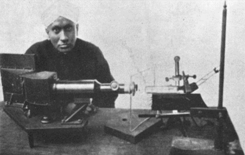
Fig. 1 C.V. Raman with his spectrometer

Raman scattering or the Raman effect is the inelastic scattering of photons by matter, meaning that there is both an exchange of energy and a change in the light’s direction. Typically this effect involves vibrational energy being gained by a molecule as incident photons from a visible laser are shifted to lower energy. This is called normal Stokes Raman scattering. If the incident photons are shifted to higher energy the process is called Anti-Stokes Raman scattering

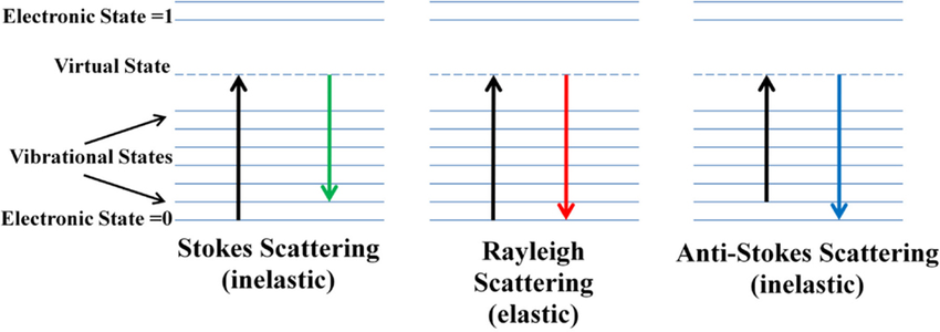
Here we can see how the incident beam produces diferent frequencies depending on the type of scattering:

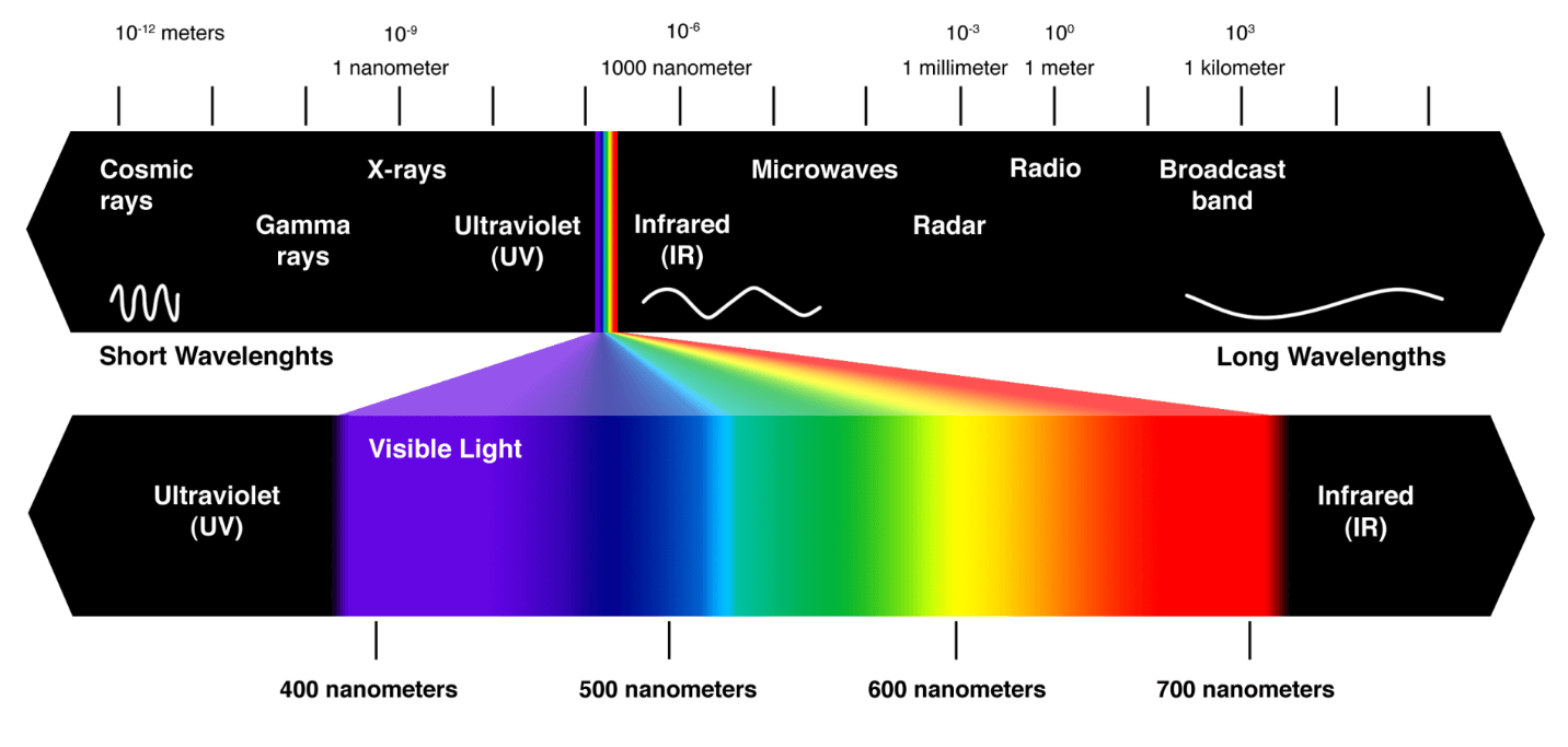
Spectrum of light

Spectroscopy techniques are available over a very wide energy range:

• Gamma rays: Mössbauer spectroscopy

• X-rays: X-ray photoelectron spectroscopy

• UV-Vis: Raman spectroscopy

• IR: IR spectroscopy

• Microwave: Electron paramagnetic resonance spectroscopy

• Radiowave: Nuclear magnetic resonance

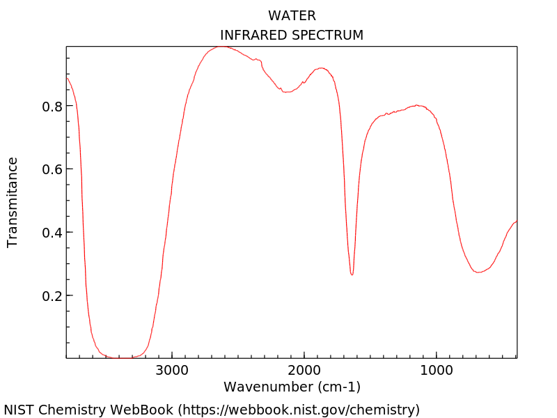
Infrared Spectroscopy

Infrared spectroscopy (IR spectroscopy) is the measurement of the interaction of infrared radiation with matter by absorption, emission, or reflection. It is used to study and identify chemical substances or functional groups. The identifications proceeds via obtaining the infrared spectrum. An IR spectrum can be visualized in a graph of infrared light absorbance (or transmittance) on the vertical axis vs the wavenumber. The wave number is a unit directric proportional to the energy.

Here we show the IR spectrum of the water, in a plot of trasmitance vs wavenumber:

Clasical approach

We can start a first approach from a clasical point of view. Imagine that we have two atoms joined by a spring, we can actually used Hook Law to derive the force that each atom experiences:

\[ F= m \frac{\partial^2 R(t) }{\partial t^2 }= \nabla_R V(R) \]

The armonic potential \(V(R)\) can be expanded in Taylor series around the equilibrium position \(R_0\):

\[ V(R) = V_0 + \frac{\partial V }{\partial R }|_{R=R_0}(R-R_0)+\frac{1}{2}\frac{\partial^2 V }{\partial R^2 }|_{R=R_0}(R-R_0)^2+... \]

Being the thrid term the spring constant \(k\)

Euler equation approach

import matplotlib.pyplot as plt
import imageio
from pylab import *

---------------------------------------------------------------------------
ModuleNotFoundError                       Traceback (most recent call last)
Cell In[1], line 2
      1 import matplotlib.pyplot as plt
----> 2 import imageio
      3 from pylab import *

ModuleNotFoundError: No module named 'imageio'

e=1 # electron charge
s=1 # interatomic distance 

m1=10 #mass 1
m1_b=1500
m2=10 #mass 2

k=10 #string constant
k2=150 #string constant
m=m1*m2/(m1+m2) #reduced mass

def vibra(part,p_0,k, m1, m2):
    FV=zeros((part,2))
    bond=2.*s
    m=m1*m2/(m1+m2)
    for at in range(0,part,2):
        d= p_0[at]-p_0[at+1] #vector distancia enlace entre un particula y su consecutiva
        r= sqrt(d[0]**2+d[1]**2) # norma del vector 
        u=d/r
        FV[at]=-k*(r-bond)*u
        FV[at+1]=-k*(-r+bond)*u
        acelv=FV/m        
    return  acelv

def graf(pn_0,vc_0,pn_k,vc_k,pn_m,vc_m):
    alpha_1=0.25
    p_0=array([[0,2],  [1, 2]]) # positions
    p_k=array([[0,0],  [1, 0]]) # positions
    p_m=array([[0,4],  [1, 4]]) # positions
    
    ax.clear()            #borra la graficar y pone otra encima
    ax.set_xlim(-3,4)  #ax tiene ese atributo porque se definió abajo
    ax.set_ylim(-3,box)  
    ax.set_xlabel("x")
    ax.set_ylabel("y")  
    
    #Change in m
    m1,m2= 10,20
    x1_m=pn_m[:,0][0]
    y1_m=pn_m[:,1][0] 
    ax.scatter(x1_m,y1_m,s=m1*50, c="blue",edgecolor="None")
    
    x2_m=pn_m[:,0][1]
    y2_m=pn_m[:,1][1] 
    ax.scatter(x2_m,y2_m,s=m2*50,c="orange",edgecolor="None")
    ax.hlines(y2_m, xmin=x1_m, xmax=x2_m, linewidth=2, color='green', label="Variation in m")
    
    ax.scatter(p_m[:,0][0],p_m[:,1][0],s=m1*50, c="blue",edgecolor="None", alpha=alpha_1)
    ax.scatter(p_m[:,0][1],p_m[:,1][1],s=m2*50, c="blue",edgecolor="None", alpha=alpha_1)
    
    
    ### Reference
    m1,m2= 10,10
    x1_0=pn_0[:,0][0]
    y1_0=pn_0[:,1][0] 
    ax.scatter(x1_0,y1_0,s=m1*50, c="blue",edgecolor="None")
    
    
    x2_0=pn_0[:,0][1]
    y2_0=pn_0[:,1][1] 
    ax.scatter(x2_0,y2_0,s=m2*50,c="orange",edgecolor="None")
    ax.hlines(y2_0, xmin=x1_0, xmax=x2_0, linewidth=2, color='black', label="Reference")
    
    ax.scatter(p_0[:,0][0],p_0[:,1][0],s=m1*50, c="blue",edgecolor="None", alpha=alpha_1)
    ax.scatter(p_0[:,0][1],p_0[:,1][1],s=m1*50, c="blue",edgecolor="None", alpha=alpha_1)
    
    #Change in k
    x1_k=pn_k[:,0][0]
    y1_k=pn_k[:,1][0] 
    ax.scatter(x1_k,y1_k,s=m1*50, c="blue",edgecolor="None")
    
    
    x2_k=pn_k[:,0][1]
    y2_k=pn_k[:,1][1] 
    ax.scatter(x2_k,y2_k,s=m2*50,c="orange",edgecolor="None")
    ax.hlines(y2_k, xmin=x1_k, xmax=x2_k, linewidth=2, color='r', label="Variation in k")
    
    ax.scatter(p_k[:,0][0],p_k[:,1][0],s=m1*50, c="blue",edgecolor="None", alpha=alpha_1)
    ax.scatter(p_k[:,0][1],p_k[:,1][1],s=m1*50, c="blue",edgecolor="None", alpha=alpha_1)
    
    leg = plt.legend(loc='lower center')
    fig.canvas.draw() #muestra la figura
    plt.show()

# #Definir parametros
%matplotlib notebook
box  = 5.0 
part = 2

# Initial conditions

v_0=array([[0, 0],  [1, 0]]) # velocities between -1 y 1
v_k=array([[0, 0],  [1, 0]]) # velocities between -1 y 1
v_m=array([[0, 0],  [1, 0]]) # velocities between -1 y 1

p_0=array([[0,2],  [1, 2]]) # positions

p_k=array([[0,0],  [1, 0]]) # positions

p_m=array([[0,4],  [1, 4]]) # positions



    
# #Building the figure
fig, ax = plt.subplots(1, 1,figsize=(6, 5))
# fig=plt.figure()
# ax=fig.add_subplot(111)  
# fig.canvas.draw()        #update the figure
    
    
dt=0.01
tiempo=0

#Start simulation

cont=0
position_0=[]
position_m=[]
position_k=[]
t=[]
while tiempo < 10:
    aV_0 = vibra(part,p_0,k,m1,m2)
    aV_k = vibra(part,p_k,k2,m1,m2)
    aV_m = vibra(part,p_m,k,m1_b,m2)
    
    vn_0 = v_0+aV_0*dt
    vn_k = v_k+aV_k*dt
    vn_m = v_m+aV_m*dt
    
    #adjust velocities
    vn_0[(vn_0>0.5)] =0.5
    vn_0[(vn_0<-0.5)]=-0.5
    
    vn_k[(vn_k>0.5)] =0.5
    vn_k[(vn_k<-0.5)]=-0.5
    
    vn_m[(vn_m>0.5)] =0.5
    vn_m[(vn_m<-0.5)]=-0.5
    
    pn_0=p_0+vn_0*dt
    pn_k=p_k+vn_k*dt
    pn_m=p_m+vn_m*dt
    
    vc_0=sqrt(vn_0[:,0]**2+vn_0[:,1]**2)
    vc_k=sqrt(vn_k[:,0]**2+vn_k[:,1]**2)
    vc_m=sqrt(vn_m[:,0]**2+vn_m[:,1]**2)
    
    cont+=1
    if cont%10==0:
        graf(pn_0,vc_0,pn_k,vc_k,pn_m,vc_m)
        
    tiempo=tiempo+dt
    p_0=pn_0
    v_0=vn_0
    
    p_k=pn_k
    v_k=vn_k
    
    p_m=pn_m
    v_m=vn_m
    position_0.append(pn_0[:,0][0])
    position_m.append(pn_m[:,0][0])
    position_k.append(pn_k[:,0][0])
    t.append(tiempo)
    


    

Coupled systems

import matplotlib.pyplot as plt
import imageio
from pylab import *

s=1
def vibra(part,p_0,k, m1, m2):
    FV=zeros((part,2))
    bond=2.*s
    m=m1*m2/(m1+m2)
    for at in range(0,part,2):
        d= p_0[at]-p_0[at+1] #vector distancia enlace entre un particula y su consecutiva
        r= sqrt(d[0]**2+d[1]**2) # norma del vector 
        u=d/r
        FV[at]=-k*(r-bond)*u
        FV[at+1]=-k*(-r+bond)*u
        acelv=FV/m        
    return  acelv

def graf(pn_0,vc_0,pn_k,vc_k,pn_m,vc_m):
    alpha_1=0.25
    p_0=array([[0,2],  [1, 2]]) # positions
    p_k=array([[0,0],  [1, 0]]) # positions
    p_m=array([[0,4],  [1, 4]]) # positions
    
    ax[0].clear()            #borra la graficar y pone otra encima
    ax[0].set_xlim(-3,4)  #ax tiene ese atributo porque se definió abajo
    ax[0].set_ylim(-3,box)  
    ax[0].set_xlabel("x")
    ax[0].set_ylabel("y")  
    
    #Change in m
    m1,m2= 10,20
    x1_m=pn_m[:,0][0]
    y1_m=pn_m[:,1][0] 
    ax[0].scatter(x1_m,y1_m,s=m1*50, c="blue",edgecolor="None")
    
    x2_m=pn_m[:,0][1]
    y2_m=pn_m[:,1][1] 
    ax[0].scatter(x2_m,y2_m,s=m2*50,c="orange",edgecolor="None")
    ax[0].hlines(y2_m, xmin=x1_m, xmax=x2_m, linewidth=2, color='green', label="Variation in m")
    
    ax[0].scatter(p_m[:,0][0],p_m[:,1][0],s=m1*50, c="blue",edgecolor="None", alpha=alpha_1)
    ax[0].scatter(p_m[:,0][1],p_m[:,1][1],s=m2*50, c="blue",edgecolor="None", alpha=alpha_1)
    
    
    ### Reference
    m1,m2= 10,10
    x1_0=pn_0[:,0][0]
    y1_0=pn_0[:,1][0] 
    ax[0].scatter(x1_0,y1_0,s=m1*50, c="blue",edgecolor="None")
    
    
    x2_0=pn_0[:,0][1]
    y2_0=pn_0[:,1][1] 
    ax[0].scatter(x2_0,y2_0,s=m2*50,c="orange",edgecolor="None")
    ax[0].hlines(y2_0, xmin=x1_0, xmax=x2_0, linewidth=2, color='black', label="Reference")
    
    ax[0].scatter(p_0[:,0][0],p_0[:,1][0],s=m1*50, c="blue",edgecolor="None", alpha=alpha_1)
    ax[0].scatter(p_0[:,0][1],p_0[:,1][1],s=m1*50, c="blue",edgecolor="None", alpha=alpha_1)
    
    #Change in k
    x1_k=pn_k[:,0][0]
    y1_k=pn_k[:,1][0] 
    ax[0].scatter(x1_k,y1_k,s=m1*50, c="blue",edgecolor="None")
    
    x2_k=pn_k[:,0][1]
    y2_k=pn_k[:,1][1] 
    ax[0].scatter(x2_k,y2_k,s=m2*50,c="orange",edgecolor="None")
    ax[0].hlines(y2_k, xmin=x1_k, xmax=x2_k, linewidth=2, color='r', label="Variation in k")
    
    ax[0].scatter(p_k[:,0][0],p_k[:,1][0],s=m1*50, c="blue",edgecolor="None", alpha=alpha_1)
    ax[0].scatter(p_k[:,0][1],p_k[:,1][1],s=m1*50, c="blue",edgecolor="None", alpha=alpha_1)
    
    
    ax[0].legend(loc='lower center')
    
    ax[1].clear() 
    ax[1].set_xlim(0,10)  #ax tiene ese atributo porque se definió abajo
    ax[1].set_ylim(-1,0)  
    ax[1].set_xlabel("time")
    ax[1].set_ylabel("x") 
    
    ax[1].plot(t,position_0, label="Reference",c="black")
    ax[1].plot(t,position_m, label="m",c="green")
    ax[1].plot(t,position_k, label="k",c="red")
    ax[1].legend()
    
    fig.canvas.draw() #muestra la figura
    plt.show()

# #Definir parametros
%matplotlib notebook
box  = 5.0 
part = 2

# Initial conditions

v_0=array([[0, 0],  [1, 0]]) # velocities between -1 y 1
v_k=array([[0, 0],  [1, 0]]) # velocities between -1 y 1
v_m=array([[0, 0],  [1, 0]]) # velocities between -1 y 1

p_0=array([[0,2],  [1, 2]]) # positions

p_k=array([[0,0],  [1, 0]]) # positions

p_m=array([[0,4],  [1, 4]]) # positions



    
# #Building the figure
fig, ax = plt.subplots(1, 2,figsize=(12, 5))
# fig=plt.figure()
# ax=fig.add_subplot(111)  
# fig.canvas.draw()        #update the figure
    
    
dt=0.01
tiempo=0

#Start simulation

cont=0
position_0=[]
position_m=[]
position_k=[]
t=[]
while tiempo < 10:
    aV_0 = vibra(part,p_0,10,10,10)
    aV_k = vibra(part,p_k,150,10,10)
    aV_m = vibra(part,p_m,10,150,10)
    
    vn_0 = v_0+aV_0*dt
    vn_k = v_k+aV_k*dt
    vn_m = v_m+aV_m*dt
    
    #adjust velocities
    vn_0[(vn_0>0.5)] =0.5
    vn_0[(vn_0<-0.5)]=-0.5
    
    vn_k[(vn_k>0.5)] =0.5
    vn_k[(vn_k<-0.5)]=-0.5
    
    vn_m[(vn_m>0.5)] =0.5
    vn_m[(vn_m<-0.5)]=-0.5
    
    pn_0=p_0+vn_0*dt
    pn_k=p_k+vn_k*dt
    pn_m=p_m+vn_m*dt
    
    vc_0=sqrt(vn_0[:,0]**2+vn_0[:,1]**2)
    vc_k=sqrt(vn_k[:,0]**2+vn_k[:,1]**2)
    vc_m=sqrt(vn_m[:,0]**2+vn_m[:,1]**2)
    
    cont+=1
    if cont%10==0:
        graf(pn_0,vc_0,pn_k,vc_k,pn_m,vc_m)
        
    tiempo=tiempo+dt
    p_0=pn_0
    v_0=vn_0
    
    p_k=pn_k
    v_k=vn_k
    
    p_m=pn_m
    v_m=vn_m
    position_0.append(pn_0[:,0][0])
    position_m.append(pn_m[:,0][0])
    position_k.append(pn_k[:,0][0])
    t.append(tiempo)

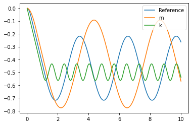
%matplotlib inline
plot(t,position_0, label="Reference")
plot(t,position_m, label="m")
plot(t,position_k, label="k")
leg = plt.legend()

import ipywidgets as widgets

widgets.RadioButtons(
    options=['pepperoni', 'pineapple', 'anchovies'],
#    value='pineapple', # Defaults to 'pineapple'
#    layout={'width': 'max-content'}, # If the items' names are long
    description='Pizza topping:',
    disabled=False
)

import plotly.express as px
data = px.data.iris()
data.head()

	sepal_length	sepal_width	petal_length	petal_width	species	species_id
0	5.1	3.5	1.4	0.2	setosa	1
1	4.9	3.0	1.4	0.2	setosa	1
2	4.7	3.2	1.3	0.2	setosa	1
3	4.6	3.1	1.5	0.2	setosa	1
4	5.0	3.6	1.4	0.2	setosa	1

import plotly.express as px
df = px.data.gapminder()
fig = px.scatter(df, x="gdpPercap", y="lifeExp", animation_frame="year", animation_group="country",
           size="pop", color="continent", hover_name="country", facet_col="continent",
           log_x=True, size_max=45, range_x=[100,100000], range_y=[25,90])
fig.show()

4961.66/256.75

19.324868549172347

from pylab import *
from ipywidgets import *

@interact(dt=(0,10,0.1), k=(1,100,5), m1=(1,100,10), m2=(1,100,10))

def Vibration(dt=0.1, k=5, m1=10, m2=10):
    s=1
    box  = 5.0 
    part = 2

    # Initial conditions

    v_0=array([[0, 0],  [1, 0]]) # velocities between -1 y 1
    p_0=array([[0, 0],  [1, 0]]) # positions


    m=m1*m2/(m1+m2) #reduced mass
    #Start simulation
    def vibra(part,p_0):
        FV=zeros((part,2))
        bond=2.*s
        for at in range(0,part,2):
            d= p_0[at]-p_0[at+1] #vector distancia enlace entre un particula y su consecutiva
            r= sqrt(d[0]**2+d[1]**2) # norma del vector 
            u=d/r
            FV[at]=-k*(r-bond)*u
            FV[at+1]=-k*(-r+bond)*u
            acelv=FV/m 
        
        return  acelv
    cont=0
    position1=[]
    position2=[]
    aV=vibra(part,p_0)
    aC=aV
    vn=v_0+aC*dt
    #adjust velocities
    vn[(vn>0.5)]=0.5
    vn[(vn<-0.5)]=-0.5

    pn=p_0+vn*dt
    vc=sqrt(vn[:,0]**2+vn[:,1]**2)

    p_0=pn
    v_0=vn
    
    position1.append(pn[:,0][0])
    position2.append(pn[:,0][1])
    
    plt.xlim(-box,box)  #ax tiene ese atributo porque se definió abajo
    plt.ylim(-box,box)  
#     ax.set_xlabel("x")
#     ax.set_ylabel("y")   
    x1=pn[:,0][0]
    y1=pn[:,1][0] 
    tiempo=linspace(0,10,len(position1))
    a=scatter(tiempo,position1,s=100,c="black",edgecolor="None")
    b=scatter(x1,y1,s=m1*50, c="blue",edgecolor="None")
    x2=pn[:,0][1]
    y2=pn[:,1][1] 
    c=scatter(x2,y2,s=m2*50,c="orange",edgecolor="None")